This post describes improvements in the dynamic range of PCM samples recovered from the PDM microphone in the SPLear™ sound level measurement module.

This is part of our series of articles on the general subject of audio signal processing from air to information.

The last post showed that we have the processing power available to improve the quality of conversion of the 1-bit per sample PDM audio bitstream from the microphone on the SPLear, moving to 16 bit PCM. This post will do some housekeeping and clean up the code, while also adding another 4 bits of dynamic range.

We began this journey in an 8-bit AVR ATTiny85 CPU. We ported that stunt to the 8-pin DIP LPC810, and then to the SPLear module based on an NXP LPC812 32-bit ARM Cortex-M0 running at 30 MHz.

Although this post continues to focus on the firmware in the SPLear, we are still compatible with scripts and programs we’ve demonstrated along the way running in a Raspberry Pi B+.

Much of the firmware and code running in the RPi has been discussed and published in past posts on this blog, and the source code is available from a public repository. The firmware and Lua program used here is checked in as [8a4059fa2f].

Revisiting Performance Measurements

I made a simple performance measurement using GPIO pins P12 and P13, driving P13 low during the SPI receive interrupt and P12 low when not waiting for the next PCM sample in the main loop.

The P12 signal is also the ISP_EN signal tested at boot which enables access to the in system programming protocol over the serial port. It can be safely used as an output, as long as it can be overridden during boot for programming.

The P13 signal is the available GPIO intended for application use. Current firmware uses P13 as the EEK signal. While in use as debug and performance measurement sonar, the application pin function must be disabled in the build.

This allows the compute time per 16 bits of PDM and per PCM sample to be directly measured with a logic analyzer or oscilloscope. I used a USBee SX to make these measurements.

The SPI interrupt period is 16/MCLK with MCLK at 500 kHz, or 32 µs. Qualitatively, three out of four interrupts are fast, and the fourth is slower. This makes sense because of the overall decimation by 64 from the 500 kHz PDM clock is achieved with a decimation by 16 in the 16-bit SPI shift register, and a further decimation by 4 before finishing the CIC and queuing a PCM sample. This section will ignore the slow interrupts other than to note that it would be a problem if they took too long.

The firmware as of the last post was consuming 3.3µs in the fastest SPI interrupts, which would be the time required for the most frequent operations of the CIC filter. That is about a 10% duty cycle, so 90% is free for the foreground and other interrupt activity such as the UART.

With that as a baseline, the first change I made was to widen the CIC accumulators to 32 bits from 16 bits. Any future filter changes that increased the bit depth further would require that, and it seemed sensible to profile that change in isolation.

The fastest SPI interrupts with 32 bit accumulators consume 3.0µs, or a 10% improvement. This speed-up is likely mostly attributable to less work required to access memory by 16 bits in a 32 bit architecture.

PCM Bit Depth

Since we have determined there is time available, we should consider the benefits from further bit depth in the PCM samples. In principle, we can go up to 31 bit PCM without any qualms.

An easy first change is to increase N from 3 to 4 in our second CIC filter cascade. That requires the addition of a fourth bank of accumulators for the integrator and the comb, or 3 more 32-bit words.

CICREG s2_sum4 = 0;
CICREG s2_comb4_1 = 0;
CICREG s2_comb4_2 = 0;

Along with the corresponding changes in SPI0_IRQHandler() to add the integrator into the cascade:

            s2_sum1 += pdmsum8[pdm&0xff] ;
            s2_sum2 += s2_sum1;
            s2_sum3 += s2_sum2;
            s2_sum4 += s2_sum3; // NEW
            s2_sum1 += pdmsum8[pdm>>8] ;
            s2_sum2 += s2_sum1;
            s2_sum3 += s2_sum2;
            s2_sum4 += s2_sum3; // NEW

And extend the comb cascade as well:

                stage4 = stage3 - s2_comb4_2;
                s2_comb4_2 = s2_comb4_1;
                s2_comb4_1 = stage3;

                // queue the finished PCM sample
                RingBuffer_Insert(&pcmring, &stage4);

The resulting CIC filter stack has the usual first block with R=8, M=1, N=1 implemented by two table lookups per SPI interrupt, followed by the second block with R=8, M=2, N=4 for a total bit depth of 20. The PCM sample rate remains 7812.5 Hz, and the theoretical peak raw SPL code value is 152 for an overall theoretical dynamic range of 114 dB.

With this implemented, the performance measurement shows the interrupt handler now requires about 4.1µs, for a 13% duty cycle. While there clearly is room for more filter calculation, we have exceeded the microphone’s signal to noise ratio at this point.

There are other minor changes that relate, notably the internal scaled SPL figure has a new peak value since it is implicitly related to the maximum absolute sample value, and that has changed from 65536 to 1048576.

#define MAXLG2SPL       152 /* 20 bit PCM */

Another related change is that the uLaw recorder mode needs to scale the PCM samples for uLaw conversion, since uLaw is defined to effectively only pass a 14 bit dynamic range, which is now a lot smaller than the 20 bit PCM samples.

Filter Quality

Bit depth is not the only measure of the quality of the PCM samples. Almost as important is the quality of the low-pass filter it implements to reject signals above the Nyquist point of the PCM sample rate.

The CIC filter is by nature a sequence of boxcar filters, which have been (cleverly) combined with decimation in a way that minimized the amount of arithmetic required.

Our CIC implementation takes that one step further, by implementing two separate decimation steps so that the first stage of the filter can be implemented by a simple table lookup which is substantially faster than all of the overheads required to extract single bit samples from a 16-bit register. By setting R to 8, we can use a 256 entry table which is a good compromise with our available ROM space where that table is stored.

Since boxcar filters are linear time invariant, our structure with two cascaded decimators can be transformed to a conventional structure with just one decimator by sliding the first decimator across the second set of filters, and adjusting the width of the moved boxcars. That is, our system as built looks like this:

(F0) --B8--/8--B16--B16--B16--B16--/8-- (F0/64)

But it can be redrawn like this:

(F0) --B8--B128--B128--B128--B128--/64-- (F0/64)

The frequency response (really, the absolute value of the impulse response) can be estimated from the response of a generic boxcar by composition:

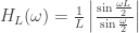
Since , we can rewrite the response in terms of f in Hz given a fixed sample rate.

So the full cascade has the form:

When plotted as gain in dB vs. log frequency ranging from 100 to 250000 Hz it looks like:

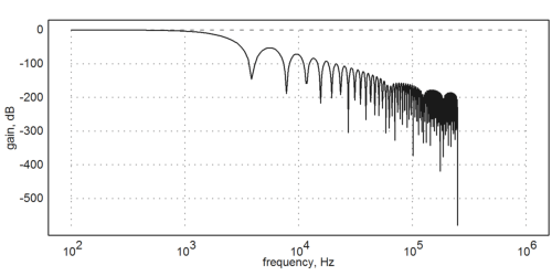
This response has 128 zeros, but when the overall decimation by 62 is considered, the output sample rate is exactly at the second zero, and the first falls inside the pass-band exactly at the Nyquist point. So what matters then is the amplitude of the first peak, which is what scales any audio above the Nyquist point aliased in to the passband. By direct evaluation, that first peak is at about -54 dB, the second at -72 dB, and the third at -84 dB.

In this figure, the red lines mark the Nyquist point and sample rate of the PCM samples at 7812.5 Hz. The green line marks the -54 dB level of the first peak in the stop band, and the plot is the filter gain in dB vs. frequency in Hz.

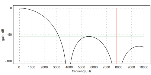
One observation is that the filter has a pretty severe roll-off. This is why any quality audio resampling filter will follow the CIC with an FIR filter stage designed to flatten the frequency response, and usually also further reduce the stop band levels.

An interesting performance question to investigate would be how many taps on an FIR filter can we afford to implement at the low sample rate, and would it be worth doing that.

For the simple measurement of environmental noise, I haven’t considered it necessary since we already are band-width limited compared to the formal definitions of either the SPL A or C weighting curves.

What Now?

The next step is to continue to find interesting things to do with the measured SPL level, which will certainly be the subject of future posts. Watch this space!

---

Please let us know what you think about the SPLear!

If you have a project involving embedded systems, micro-controllers, electronics design, audio, video, or more we can help. Check out our main site and call or email us with your needs. No project is too small!

+1 626 303-1602
Cheshire Engineering Corp.
120 W Olive Ave
Monrovia, CA 91016

---

(Written with StackEdit.)